I've been at eVSM for three and a half years, and have added a ton of cool functionality to the software.
Hardly anyone realizes this.
For that reason and many others, we've been focusing our attention on delivering a great self-paced learning environment for eVSM v9, which will all be released at the start of 2016. That's assuming everything goes well, anyway.
This new capability will allow us to first deliver great training for our main quick stencils, but over time we'll add more and more advanced tutorials that will expose many of the great tools we've worked on but never fully delivered.
Learn more at our LinkedIn user group:
https://www.linkedin.com/grp/post/3382476-6054686331278290948
Friday, October 2, 2015

Thursday, September 17, 2015
Transactional Demand River
Part of our improvements to the Transactional Pro capability in eVSM included an enhancement to our line thickness visualization gadget. Each green arrow in our transactional map now carries a variable for the demand flowing through it. The gadget uses this data to determine the line thickness.
So, the practical upshot is that it's easy to see how much demand is flowing through a system, even when there rework and splits/merges are involved. When this was shown to an improvement team, they ended up naming this the 'demand river', as it is somewhat akin to water flowing, splitting off, and flowing back together.
Below is an example future state map for a clinical approval process. The goal of the future state design was to make most of the requests finish with the shortest total lead time possible. We used the demand river to help show the improvement in routings. The big fat lines upstream flow quickly through some decision processes, and split off so that the less-common long-lead items are identified early, and the quick/easy items get approved as quickly as possible.

The underlying data is of course of great interest, but it's absolutely necessary to be able to show it to people visually. Great visualizations like the demand river really help people to understand what the map is showing, which makes it easier for people to reconcile that with the real world. This includes being able to point out mistakes in the map (and in the author's conception of the system) much easier than if you had to try and understand a bunch of data points.
Wednesday, September 16, 2015
Transactional Pro Update
My last post was back in March, and detailed some of the work we did for transactional value stream mapping and analysis. Shortly after that post, we revisited the stencil with some ideas on improving usability and performance.
Long story short, we changed the route table so that you could now have multiple route tables on a single page, and each one could be filtered to show only what you're interested in. For instance, you could easily see just the routes that represent more than X % of the total flow, or cost, in the system.
You can also configure a route table to show only certain variables, and leave out what you don't want, and sort by whatever variable you want.
We also re-factored the software so that you no longer have to re-run the simulation in order to re-draw the route table. You can just add route tables, slice and dice them, iterating quickly, without having to re-run the simulation.
Check out the tutorial for more information, and if needed get a trial download.
Long story short, we changed the route table so that you could now have multiple route tables on a single page, and each one could be filtered to show only what you're interested in. For instance, you could easily see just the routes that represent more than X % of the total flow, or cost, in the system.
You can also configure a route table to show only certain variables, and leave out what you don't want, and sort by whatever variable you want.
We also re-factored the software so that you no longer have to re-run the simulation in order to re-draw the route table. You can just add route tables, slice and dice them, iterating quickly, without having to re-run the simulation.
Check out the tutorial for more information, and if needed get a trial download.
Thursday, March 19, 2015
eVSM Quick Transactional Pro
Last year we had a look at our Transactional mapping stencil, and compared its capabilities with example maps from Karen Martin & Mike Osterling's excellent Value Stream Mapping book. We were easilty able to replicate them in eVSM, though we found some of the calculations differed, mainly how lead time is calculated.
Our Quick Manufacturing stencil calculates lead time for inventories based on Little's Law, which is totally reasonable and appropriate for discrete manufacturing. Rather than get into the nuances here, I guess I'll just link Karen's post on the topic because this post is supposed to be about what we did about our findings with the Transactional stencil.
So we looked at everything we did for mapping transactional value streams, and decided the biggest deficiency we had was in handling rework loops. We provided a very basic calculation for rework and left it at that, not even really having it impact lead time, just cost.
In the end we decided to try allowing loops in analyzing transactional value streams. We also had started implementing some calculations for parallel processing in the old Quick Transactional stencil, but wanted to provide full support for it going forward.
What came out of all this work is a new stencil, and a lot of supporting code, called Quick Transactional Pro. The stencil allows you to draw a transactional map with constructs available for multiple rework loops, document splitting and merging, and various termination points. We used constructs from Business Process Modeling Notation (BPMN), specifically: split, merge, and terminate centers.
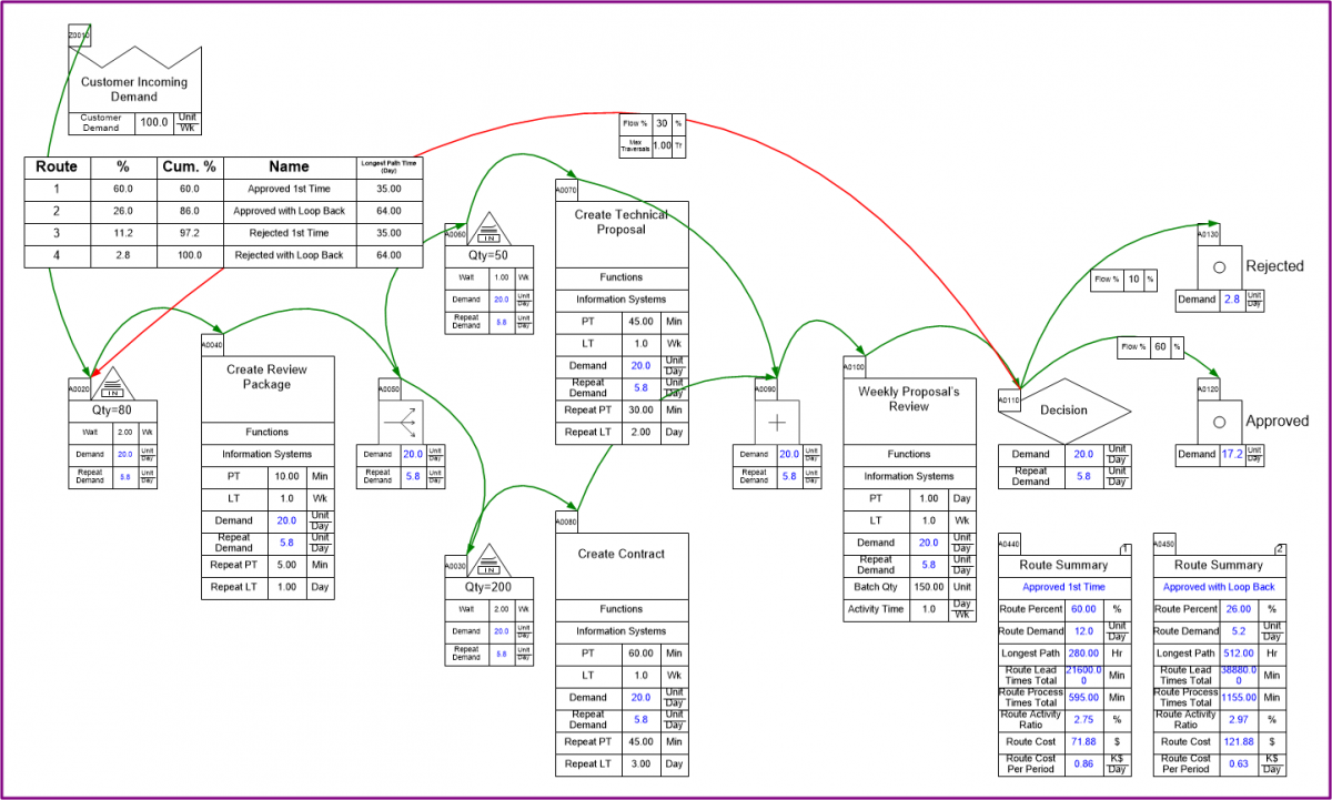
We tried to make the modeling job as easy as possible, so we end up assuming that the repeat process and lead times are the same as the first-time, but you can add repeat time data when the repeat processing is faster (or slower) than the first time through a process.
Once the map is built you use the Solve tool, which works a bit differently than normal on these types of maps. Rather than perform static Excel calculations, like all our other stencils, we run a three-stage solve. The first stage pre-populates some simple calculations, needed for the second phase. The second phase is a small scale simulation, where we generate some number of 'flow tokens' (250 by default), and send them one-by-one through the value stream. We track the whole route each token takes, and identify every unique route taken. We also count the number of tokens that follow each route.
This flow data is then passed to the third phase of the solve, which uses that flow data first to calculate the First-Time and Repeat demand at every single center in the value stream. This allows us to get a better idea of the actual demand faced by different resources in the value stream, and what capacity is required to serve demand.
The flow data also gets used in the third phase, to give route-specific lead times. We use the flow data to generate what we call a Route Table, which shows all the unique routes identified by the simulation, sorted from highest percentage of flow to the lowest.


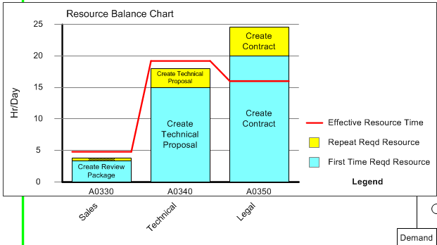
You can also assign resources across processes, and see a balance chart:
Our Quick Manufacturing stencil calculates lead time for inventories based on Little's Law, which is totally reasonable and appropriate for discrete manufacturing. Rather than get into the nuances here, I guess I'll just link Karen's post on the topic because this post is supposed to be about what we did about our findings with the Transactional stencil.
So we looked at everything we did for mapping transactional value streams, and decided the biggest deficiency we had was in handling rework loops. We provided a very basic calculation for rework and left it at that, not even really having it impact lead time, just cost.
In the end we decided to try allowing loops in analyzing transactional value streams. We also had started implementing some calculations for parallel processing in the old Quick Transactional stencil, but wanted to provide full support for it going forward.
What came out of all this work is a new stencil, and a lot of supporting code, called Quick Transactional Pro. The stencil allows you to draw a transactional map with constructs available for multiple rework loops, document splitting and merging, and various termination points. We used constructs from Business Process Modeling Notation (BPMN), specifically: split, merge, and terminate centers.
We tried to make the modeling job as easy as possible, so we end up assuming that the repeat process and lead times are the same as the first-time, but you can add repeat time data when the repeat processing is faster (or slower) than the first time through a process.
Once the map is built you use the Solve tool, which works a bit differently than normal on these types of maps. Rather than perform static Excel calculations, like all our other stencils, we run a three-stage solve. The first stage pre-populates some simple calculations, needed for the second phase. The second phase is a small scale simulation, where we generate some number of 'flow tokens' (250 by default), and send them one-by-one through the value stream. We track the whole route each token takes, and identify every unique route taken. We also count the number of tokens that follow each route.
This flow data is then passed to the third phase of the solve, which uses that flow data first to calculate the First-Time and Repeat demand at every single center in the value stream. This allows us to get a better idea of the actual demand faced by different resources in the value stream, and what capacity is required to serve demand.
The flow data also gets used in the third phase, to give route-specific lead times. We use the flow data to generate what we call a Route Table, which shows all the unique routes identified by the simulation, sorted from highest percentage of flow to the lowest.
The route table is a great way to tell at a glance what are the most common routes through the value stream, and their corresponding lead times. You can also drill down a little further into a single route with the Route Summary, which shows costs associated with a route, the demand, and the Activity Ratio, which is the ratio of Activity Time to Lead Time.
You can right-click on any row and view what activities are part of the route, and you can also see an animated view of the 'token' flowing through. If you want to know your first-pass C&A you would find the route where tokens flow through without rework, and get the flow %.
We also include a few charts, including a lead time ladder chart showing lead components for different routes:
This stencil has been out since last summer, but I've only now gotten around to talking about it. There are a few more exciting new tools in eVSM that I hope to write about sooner.
Quick Transactional Pro is a new way of thinking about mapping transactional value streams, and I can't think of an easier way to see transactional systems when there are loops and parallel processing.
Give eVSM v8 a try now, which includes Quick Transactional Pro. If it's been a while since you've tried eVSM, try it again.
Wednesday, July 2, 2014
eVSM v7 released
We released v7 of eVSM about six months ago, but I haven't posted anything about it here yet. I usually wait until we have a quiet time to go about posting about this stuff, but we've been going pretty fast and heavy on some new functionality, as well as stabilizing migration of older maps. Bad excuse, but there it is.
Anyway, things still aren't quiet here, as we're moving fast on a couple new features, and now we're using secret codenames for projects: Honeyduke, SafetyWeb, and Bertie Bott. All pretty cool functionality that are coming into the product as kind of beta features during v7, and will be finalized in v8 early next year. The code names are coming mostly from Harry Potter, but I think we'll have some Douglas Adams and Lord of the Rings code names too.
v7 is already at its 18th release, so here's a short list of what we've added so far this year:
Anyway, things still aren't quiet here, as we're moving fast on a couple new features, and now we're using secret codenames for projects: Honeyduke, SafetyWeb, and Bertie Bott. All pretty cool functionality that are coming into the product as kind of beta features during v7, and will be finalized in v8 early next year. The code names are coming mostly from Harry Potter, but I think we'll have some Douglas Adams and Lord of the Rings code names too.
v7 is already at its 18th release, so here's a short list of what we've added so far this year:
- New Metric/US units selection - add the Name/Unit data for a map and you now choose what units to use
- Added the Map Copy button back to the ribbon, should be a nice fast way to copy a map to another page
- Added a Stack Help button to help you pick the right icon for a transmit/transport/etc.. shape
- Added Icon Search to help you find a master you want to use. So if you're looking for Changeover, just search that and you'll see what shapes are associated with Changeover.
- Reworked Kaizen/Starburst system, allowing you to pick what data you are interested in, and edit only those fields with bidirectional Excel export/import.
- Revamped the Sketcher Picture Import workflow to make it easier to scale an imported wall map picture
- Added a new MultiAdd quick master type, which basically allows you to assign default addons when you drop say an Activity Center MultiAdd.
- Honeyduke Solve, which is essentially a flow simulation for tokens (work items, patients, whatever might be moving through the value stream). This simulation gives us the ability to calculate demand in the presence of rework loops, document/workflow splits and merges. Very exciting. Use the Quick Transactional Pro stencil to try it out. We might bring this to other stencils but for now it's focused on Office/Healthcare applications.
- Performance has been a big focus in a lot of areas, which is not something most people will probably notice, but my hope is using eVSM will feel smoother and faster going forward, not clunkier and slower.
I wish I could say we have countless other changes, but I can't since I have over 1100 changes logged since the final v6 release. Regardless there are a lot of tweaks, fixes, and improvements and I would encourage you to try, buy, or upgrade to the latest release of eVSM.
We've done a lot of work under the covers, too, to help make the product more reliable. This includes a lot of work on tools to help us manage code development, profiling, and automated testing. I will write a little about this in the future. The next big challenge will be the Bertie Bott project, which I can't elaborate on, but it could be very useful. Possibly more useful than Honeyduke, and Honeyduke is very cool.
Thursday, February 6, 2014
Mailbox App for Demand Leveling
For about a year now, I've been using the Mailbox app on my iPhone and iPad, to manage my work to do list. I know there are a lot of great to do list apps out there (with Trello being my favorite), but the simplest way for me to work is to use my email inbox as my to do list.
I'm usually pretty insistent on maintaining Inbox Zero with my email account, so using it as my to do list also encourages me to get everything I need to get done, done.
But some days I just get slammed with emails from my eVSM colleagues, as well as customer support issues, on top of my usual list of subscription emails. My inbox ends up with a lot more than zero emails in it.
So I have started using the Mailbox app, which is awesome. It will "snooze" an email until a time/day you specify, with a buttery smooth user interface. I actually had a similar system in place that I had put together using Google Apps Script, but it required me to move items into different named folders (like 'wait 1 day', 'wait 1 week', etc...). Mailbox lets me just move something to:
I'm usually pretty insistent on maintaining Inbox Zero with my email account, so using it as my to do list also encourages me to get everything I need to get done, done.
But some days I just get slammed with emails from my eVSM colleagues, as well as customer support issues, on top of my usual list of subscription emails. My inbox ends up with a lot more than zero emails in it.
So I have started using the Mailbox app, which is awesome. It will "snooze" an email until a time/day you specify, with a buttery smooth user interface. I actually had a similar system in place that I had put together using Google Apps Script, but it required me to move items into different named folders (like 'wait 1 day', 'wait 1 week', etc...). Mailbox lets me just move something to:
- Later Today (3 hours later, I believe)
- This Evening
- Tomorrow (Morning)
- This Weekend
- Next Week
- Next Month
- Someday (not sure when that is - 3 months?)
- or a specific Date/Time
and at that time, Mailbox will move the email back to my inbox. Until then, it's hidden in a Gmail folder.
So now when my inbox is flooded with emails, I just open the app up and start snoozing emails and clearing the inbox. It's pretty easy to pick these different snooze times so that the emails come back in the order I want to work on them. And sometimes when an email comes back, I snooze it again immediately.
But this app provides a beautifully easy way for me to not only keep my inbox (and my mind) clear of clutter, but also makes it really easy for me to follow up on emails weeks later, when there is zero chance I'd remember to do it myself.
I find myself much more capable at focusing on my work when I only have one or two or three tasks looking at me in my email inbox, rather than trying to constantly re-sort all those emails in my head when I check my email. It would be nice if I could snooze emails from my email client, or even a web app, but I'm fine with using one of my iOS gadgets to do it.
Thursday, January 30, 2014
IFTTT as a Lean Enabling Tool
A few weeks ago we had a bad cold snap in Connecticut, and a few of my pipes froze. The pipes froze not just because of the sub 0F temperatures, but also because I had my wood stove running pretty hard throughout the cold. Because it was so warm in my house from the wood stove, the thermostat in my hall never turned the furnace on, which would have circulated hot water through my baseboard heating system. Instead, the water sat in the pipes and cooled down, and eventually froze.
While I waited for the pipes to thaw, and also while I was repairing one of them, which had burst and started spewing hot water into my basement, I thought about how I could prevent this from happening again.
I could have bought electric heaters for the pipes, which would have been a lot of expense and time buying and installing them. I could also just not run my wood stove, which would mean I'd use more oil than I had been, which would also be pretty expensive.
Instead of spending money on the problem, I decided to try to implement some standard work for handling the cold in my house. I know how silly that sounds, but bear with me. It doesn't get this cold very often in CT (although it has been fairly often this winter), so I knew I'd get careless some night or not pay attention to the forecast, and I'd be back to doing extremely bad pipe soldering jobs (actually, if it happens again I'm going to use PEX).
So I turned to a very cool web-based tool called IFTTT (IF This Then That), which is a service that monitors any of a huge number of different "conditions." The condition can be generated by (currently) around 70 different web services like Facebook, GMail, or Pinboard. When a condition is satisfied (like a new tweet to you, or a new email), you can then have some action run, again against this huge list of web services.
The really cool part of IFTTT is that they have some links into the real world, and not just messaging services. One example is the WeMo switch system, so you can have a lamp turn on when someone sends you an email (who wouldn't want that?). They're also hooked into the weather forecast, which is why I mention the pipes freezing.
So what I ended up doing was, setting up a trigger condition, to send me an email when the forecasted temperature is supposed to be less than 8 degrees Fahrenheit, which is a few degrees above where I've ever had problems with pipes freezing. But I built a list of "tasks" to do when the weather is going to be cold, basically:
While I waited for the pipes to thaw, and also while I was repairing one of them, which had burst and started spewing hot water into my basement, I thought about how I could prevent this from happening again.
I could have bought electric heaters for the pipes, which would have been a lot of expense and time buying and installing them. I could also just not run my wood stove, which would mean I'd use more oil than I had been, which would also be pretty expensive.
Instead of spending money on the problem, I decided to try to implement some standard work for handling the cold in my house. I know how silly that sounds, but bear with me. It doesn't get this cold very often in CT (although it has been fairly often this winter), so I knew I'd get careless some night or not pay attention to the forecast, and I'd be back to doing extremely bad pipe soldering jobs (actually, if it happens again I'm going to use PEX).
So I turned to a very cool web-based tool called IFTTT (IF This Then That), which is a service that monitors any of a huge number of different "conditions." The condition can be generated by (currently) around 70 different web services like Facebook, GMail, or Pinboard. When a condition is satisfied (like a new tweet to you, or a new email), you can then have some action run, again against this huge list of web services.
The really cool part of IFTTT is that they have some links into the real world, and not just messaging services. One example is the WeMo switch system, so you can have a lamp turn on when someone sends you an email (who wouldn't want that?). They're also hooked into the weather forecast, which is why I mention the pipes freezing.
So what I ended up doing was, setting up a trigger condition, to send me an email when the forecasted temperature is supposed to be less than 8 degrees Fahrenheit, which is a few degrees above where I've ever had problems with pipes freezing. But I built a list of "tasks" to do when the weather is going to be cold, basically:
- Make sure my basement has good airflow, so my cedar closet gets good air flow (that's where the burst happened)
- Make sure I turn the thermostat on before I go to sleep, to warm the pipes
- Lay off the wood stove a little bit, so the thermostat is able to come on through the night
Now, I don't have to spend any mental effort on what the weather is like, I just let the IFTTT service keep an eye on things and tell me only on days when I have to worry about it. I actually set the alert up to send me an alert when the forecast is for less than 8 degrees, and then again when the temperature actually dips that low.
And really, I feel like the optimal set up for me would be to have something like the Nest thermostat, but have it controlled via the IFTTT service or something similar. I'd like it to go into a different mode when the temperature outside my house drops, and no matter what the temperature in the house, just circulate the water in the pipes every hour or two. If only there was an IFTTT trigger for when Nest integrates with IFTTT. And I just looked, and they actually have a trigger for new channels. Crazy.
So after all that, my point is, you should have a look at IFTTT.com, and think about whether there is some trigger you could use to alert you so you don't miss something. Or maybe set up a trigger so when your most important client sends you a message, that lamp does turn on. Why not? How much is it worth to make them happy? Also, that WeMo system has a motion detector, so you could set IFTTT up to text you when someone trips that motion sensor.
I've actually thought about this topic quite a lot over the last few years, after noticing that a lot of the reason that organizations struggle with change because they let processes stagnate for years regardless of changes in conditions. So I've always wanted a tool that would let me input the conditions that affected some business decision, and once those conditions change, they tell me to re-evaluate the conditions and update my processes. That's what's exciting about IFTTT, because as they add more and more of these trigger channels, the tool I want so badly gets closer and closer to fruition.
So that's why I say IFTTT is a lean-enabling tool. It lets you focus on other things, but makes sure you don't miss out on something important.
Tuesday, January 7, 2014
Monte-Carlo (sort of) Simulation in eVSM
I have been talking a little about new enhancements to the calculation engine in eVSM. One very exciting development here is what we are calling Variational Solve. We added this because we know that variation is a huge source of waste in most value streams. We thought that being able to visualize variation on a map would help in reducing or eliminating it.
So there are a few different parts to the variational solve. The first is somehow getting variation data into eVSM for the calculation engine to use. The second is actually calculating variation in the map. And the last part is visualizing it. I'll go into all three in this post.
We wanted to make variation data input as easy as possible, and we settled on using Distribution shapes, which you glue onto variables in eVSM. We included Normal, Uniform, Triangular, and Exponential distributions out of the box. For those with simulation backgrounds, this is a very small subset of what's available in most commercial simulation packages, but we felt that most of our users wouldn't want to bother with distribution fitting software to feed into eVSM. We kept it simple and hope that you can model whatever you need with the distributions we've made available. For everything else, we've also provided a List distribution, which simply stores a list of values inside the shape.
So to use any of these distributions, you drag out one of the distribution shapes and glue it onto the variable you're applying the distribution to.

Each distribution has a set of parameters, which are just sub-shapes for the distribution shape. You can hold your mouse over the sub shape for any parameter, and Visio will display the parameter name. I've also summarized the parameters below:

So there are a few different parts to the variational solve. The first is somehow getting variation data into eVSM for the calculation engine to use. The second is actually calculating variation in the map. And the last part is visualizing it. I'll go into all three in this post.
We wanted to make variation data input as easy as possible, and we settled on using Distribution shapes, which you glue onto variables in eVSM. We included Normal, Uniform, Triangular, and Exponential distributions out of the box. For those with simulation backgrounds, this is a very small subset of what's available in most commercial simulation packages, but we felt that most of our users wouldn't want to bother with distribution fitting software to feed into eVSM. We kept it simple and hope that you can model whatever you need with the distributions we've made available. For everything else, we've also provided a List distribution, which simply stores a list of values inside the shape.
So to use any of these distributions, you drag out one of the distribution shapes and glue it onto the variable you're applying the distribution to.
- Uniform - the top value is the minimum value, bottom is the maximum
- Triangular - a is the median/central tendency, b is the maximum, and c is the minimum
- Exponential - l is the lambda parameter, or the mean
- Normal - m is the mean, sd is the standard deviation
The List Distribution is handled differently. To enter values into the list distribution, right click it and and select 'Edit List Values'. There you can enter values one by one, or paste them from Excel.
Next, you would want to decide what calculated values to measure the variation on. For instance, you might want to know how the lead time varies with random inputs on inventories or cycle times. So you would drag an Output Variation shape out from the main eVSM stencil and glue it onto the Lead Time NVU in a Time Summary. When you run a simulation, eVSM will then store every observation of the calculated value within the Output Variation shape, and make that data available for analysis.
Now, with your variable inputs defined, and your outputs, you would run the Variational Solve by first clicking the button of the same name in the eVSM ribbon. This will bring up the Variational Solve dialog, where you enter the number of iterations to run. The rule of thumb here is to increase the number of iterations with increasing amounts of variation in the system.

Variational Solve icon
So after you run a simulation with some number of replications, you want to analyze and visualize the results. As I mentioned before, the solve engine will store all observations of calculated values into glued-on Output Variation shapes. We also store the samples used for each distribution within the distribution shape. Lastly, you can turn an Output Variation shape into an input distribution, by right clicking the shape and selecting that option.
Any distribution or Output Variation shape has a right-mouse option for plotting a histogram of observations, too. This allows you to look at the variability of the distribution: how big the spread is and also what shape the data observations take.
You can also right-click on any variable shape and plot the distributions of all NVU's with that name. An example of this can be seen below, where we have process A0070 having a cycle time with a mean of 10 minutes, and A0030 with a mean of 20 minutes. You can see though that the 20 minute cycle time is probably more desirable, since the variability is so much smaller, even though it's a longer time. Instead of trying to reduce the 20 minute time, it would serve the value stream better to reduce the amount of variation on the 10 minute cycle time.

You can also view a list of all samples, either for a distribution or output variation shape, and export that to Excel for other analysis.
We've also provided a shape called the Variation Percentile, which is actually for use in static calculations. What it does is, samples the input values for a calculated values, at a certain percentile. So if for instance you wanted to know the minimum sum of cycle times on a map, you can do that with the variation percentile shape. So you would have to write a managed equation that just sums up all the Cycle Time values on the map, and samples, say, the 5th percentile value for each one.
Rather than write a managed equation, though, you can instead use a Data Target shape, since each NVU is an implicit data source. So this is all you'd have to do to get the sum of all 5th percentile NVU values for cycle time:

Any distribution or Output Variation shape has a right-mouse option for plotting a histogram of observations, too. This allows you to look at the variability of the distribution: how big the spread is and also what shape the data observations take.
You can also right-click on any variable shape and plot the distributions of all NVU's with that name. An example of this can be seen below, where we have process A0070 having a cycle time with a mean of 10 minutes, and A0030 with a mean of 20 minutes. You can see though that the 20 minute cycle time is probably more desirable, since the variability is so much smaller, even though it's a longer time. Instead of trying to reduce the 20 minute time, it would serve the value stream better to reduce the amount of variation on the 10 minute cycle time.

We've also provided a shape called the Variation Percentile, which is actually for use in static calculations. What it does is, samples the input values for a calculated values, at a certain percentile. So if for instance you wanted to know the minimum sum of cycle times on a map, you can do that with the variation percentile shape. So you would have to write a managed equation that just sums up all the Cycle Time values on the map, and samples, say, the 5th percentile value for each one.
Rather than write a managed equation, though, you can instead use a Data Target shape, since each NVU is an implicit data source. So this is all you'd have to do to get the sum of all 5th percentile NVU values for cycle time:

So these variational tools were created in the hopes of allowing you to easily add variational data to a value stream map, and visualize that. We don't want to get into a full-on simulation tool, since even the modern, well-developed ones like Simio are still pretty hard to understand and use. We wanted to start with a minimum functionality that most of our users can use and do something with.
One thing to keep in mind with this variational solve is, any of these calculated values can be sampling independent random variables from across the map. For instance, if you're keeping the output variation for Lead Time, and you have a bunch of inventory centers, those inventories are going to fluctuate randomly independent of each other. In real life this may not be the case. It's possible inventories can be dependent on one another, and so the variational solve might then not give a very valid result. So one thing you'll have to think about is, does this limitation make the answer more conservative, or more optimistic?
So if you do find that you're mapping a system and have some variability to address, try using the variational capabilities in eVSM v6. Visualize the sources of variation on the map, and use that to start working out how to reduce variation, and see how that can affect your future state. Let us know how it goes, and if there are any limits you run into, and we will be happy to work out how to move past them.
Friday, January 3, 2014
Lean guitar-making
I'm probably late hearing this, but I just listened to the Alton Brown Cast where he interviewed Bob Taylor from Taylor Guitars. They talk about quite a lot, including sustainability, and lean manufacturing for guitars. Bob talks about when they started building guitars, they would try to build a batch of 10 guitars to optimize for setup time, but would usually come in much later than planned, with only 5 guitars finished.
So they visited a luthier who had maybe 10 guitars going at once, but at different stages, so that instead of finishing 10 guitars every 10 days, he got one guitar done every day. This meant he had to do more setups, but repeating the setup so often actually let him get really good at the setup job.
The thing I really like about Taylor's approach, is that it's lean without having to call it lean, they're doing the right things and just getting things done. That's the best way to do it.
It's a great listen, especially if you're a fan of Alton Brown, like me.
Alton Brown Cast
So they visited a luthier who had maybe 10 guitars going at once, but at different stages, so that instead of finishing 10 guitars every 10 days, he got one guitar done every day. This meant he had to do more setups, but repeating the setup so often actually let him get really good at the setup job.
The thing I really like about Taylor's approach, is that it's lean without having to call it lean, they're doing the right things and just getting things done. That's the best way to do it.
It's a great listen, especially if you're a fan of Alton Brown, like me.
Alton Brown Cast
Monday, December 30, 2013
eVSM Managed Equations - Part 2 (and the Calculation Explorer)
OK so in part 1 of this post, I talked about what eVSM managed equations are and how the basic ones work. In this post, I'd like to briefly go over the arrow-based selectors for managed equations, but in all honesty they are probably beyond the scope of what most of our users will want to do with them.
So I'll start with a very busy image showing a few things of real interest:

The first thing I want to point out is the "Calculation Explorer" dialog. This dialog actually has shipped with, I think, every release of v6, at least those with the Beta Toolbar. The calculation explorer actually resides within the Developer ribbon, so definitely be careful in there. But getting the developer ribbon is done the same as getting the Beta Toolbar, so go read that if you need to get that working.
The Calculation Explorer is a neat utility. What it does is, first adds a simple unstyled text box onto the page for each hidden variable on the map, and then it runs through a partial Solve cycle, just enough to pick up the dependency tree of the map. Excel provides similar buttons, for exploring the dependency tree of a worksheet.
Anyway, this dialog exists for the sole purpose of visualizing the relationships between variables on the map. It is very useful in debugging calculations, especially since it prints out messages from the Solve engine, explaining some of the decisions it has made about linking different variables on the map.
Now, the reason the Calculation Explorer is in a post about managed equations is that we display a simplified view of the managed equation for the selected variable. This, combined with the Solve trace output, can tell us much about how a managed equation got applied (or skipped).
In the image above, you can see I've selected the Resource Usage NVU on the Pipe Arrow between tags A0030 and A0040. Actually you can't see the selection in the image, but just look at where the second text block in the top center of the Visio window. When I selected that text block, the dialog displayed the equation, which is 'SP[Resource PT] * DPC[Computed Demand]', and when I clicked the "Show Precedents" button, it drew arrows to the corresponding NVU's. So you'll see that the Resource PT NVU that is being pointed to is on the Same Pipe, which is what SP stands for. You'll also see that the Computed Demand variable is on the activity Downstream from the Pipe, at the end of the Connection, hence DPC - Downstream Pipe Connect. So this selects an NVU from the center on the head end of Pipe Arrow. UPC selects from the center at the tail of the arrow. UC and DC work the exact same way, except that they apply to Tag Sequence arrows rather than Pipes.
The SP, or Same Pipe, has an analog in the SA selector, which is Same Arrow, and applies to Tag Sequence arrows.

This image doesn't show real equations in Quick Mfg like the first image does, but it does illustrate the remaining selectors. The UPTS/DPTS selectors let you get a variable from a center on the other end of a pipe arrow (or sequence arrow, using UTS/DTS). UPS/DPS let you select a variable from the pipe arrow data set, and UAS/DAS let you do the same with Tag Sequence arrows.
There is no denying that these selectors can be a bit confusing. The good thing is our stencil designers understand this very well and most of our users just get to use the centers and not worry about it. If you want to build your own managed equations, I hope these two posts might help you better to understand how to go about doing that. Or, if you're just curious how we build our calculations, this should show you. I do encourage you to explore a map you have at some point, using that Calculation Explorer utility.
So I'll start with a very busy image showing a few things of real interest:

The first thing I want to point out is the "Calculation Explorer" dialog. This dialog actually has shipped with, I think, every release of v6, at least those with the Beta Toolbar. The calculation explorer actually resides within the Developer ribbon, so definitely be careful in there. But getting the developer ribbon is done the same as getting the Beta Toolbar, so go read that if you need to get that working.
The Calculation Explorer is a neat utility. What it does is, first adds a simple unstyled text box onto the page for each hidden variable on the map, and then it runs through a partial Solve cycle, just enough to pick up the dependency tree of the map. Excel provides similar buttons, for exploring the dependency tree of a worksheet.
Anyway, this dialog exists for the sole purpose of visualizing the relationships between variables on the map. It is very useful in debugging calculations, especially since it prints out messages from the Solve engine, explaining some of the decisions it has made about linking different variables on the map.
Now, the reason the Calculation Explorer is in a post about managed equations is that we display a simplified view of the managed equation for the selected variable. This, combined with the Solve trace output, can tell us much about how a managed equation got applied (or skipped).
In the image above, you can see I've selected the Resource Usage NVU on the Pipe Arrow between tags A0030 and A0040. Actually you can't see the selection in the image, but just look at where the second text block in the top center of the Visio window. When I selected that text block, the dialog displayed the equation, which is 'SP[Resource PT] * DPC[Computed Demand]', and when I clicked the "Show Precedents" button, it drew arrows to the corresponding NVU's. So you'll see that the Resource PT NVU that is being pointed to is on the Same Pipe, which is what SP stands for. You'll also see that the Computed Demand variable is on the activity Downstream from the Pipe, at the end of the Connection, hence DPC - Downstream Pipe Connect. So this selects an NVU from the center on the head end of Pipe Arrow. UPC selects from the center at the tail of the arrow. UC and DC work the exact same way, except that they apply to Tag Sequence arrows rather than Pipes.
The SP, or Same Pipe, has an analog in the SA selector, which is Same Arrow, and applies to Tag Sequence arrows.

This image doesn't show real equations in Quick Mfg like the first image does, but it does illustrate the remaining selectors. The UPTS/DPTS selectors let you get a variable from a center on the other end of a pipe arrow (or sequence arrow, using UTS/DTS). UPS/DPS let you select a variable from the pipe arrow data set, and UAS/DAS let you do the same with Tag Sequence arrows.
There is no denying that these selectors can be a bit confusing. The good thing is our stencil designers understand this very well and most of our users just get to use the centers and not worry about it. If you want to build your own managed equations, I hope these two posts might help you better to understand how to go about doing that. Or, if you're just curious how we build our calculations, this should show you. I do encourage you to explore a map you have at some point, using that Calculation Explorer utility.
Monday, December 23, 2013
Source / Target for sub-modelling
Since eVSM v6.15 or so, we've had a fairly powerful (and I hope, simple to understand) capability called Source/Target. What it does, simply, is allow you to use the value of a variable in one map, as the value of a variable on another page in the same Visio document.
There is some initial setup required, which tells eVSM to search other pages for source/target links when you click the eVSM Calculator button. We call this the page scope of the map. To set up page scope, click the Name Unit Manager button in the eVSM toolbar/ribbon, and find the "Source/Target Pages" button on the bottom of the NUM dialog box.
The dialog just lists all the pages in the current document, and selecting a page will make the eVSM Calculator search the page for data sources and targets to match up.

So with that out of the way, Source/Target works by first defining named data sources. The pink shape in the image above is a data source, which you just glue onto an NVU to link to the value. You then change the text from XX to whatever name you want to give it (can be a number, or any kind of text).
Then, to use the value from a data source, you attach the light blue data target to another NVU, and set its text to the same as your data source.
You can actually have many data sources with the same name, though that means your data target(s) will need to know how to "aggregate" the multiple values. By default, we just return the Sum of all the values. But you can actually take the average, minimum, or maximum value too.
There's also an undocumented feature here, that lets you use simple wild cards to match sources to a target. So if you named all your different sources such that any starting with the letter A is a certain group, and B is another, etc..., you'd be able to set the target text to A* and that would pick up anything starting with the letter A.
There's also a not-so undocumented feature, which is that every NVU on the map has an implied Data Source, with the text set to the NVU name. That means if you wanted to get the sum of all the NVU's with a certain name, you could just add a data target and set its text to the NVU name. This helps you out of having to write very simple managed equations.
We also provide the option of filtering by the path(s) of the parent center, and we provide a dialog for exploring all the sources that feed a target. That dialog actually does link to the dialog for setting the page link scope.
If you have any questions on this leave a comment or contact me, I'm happy to discuss...
There is some initial setup required, which tells eVSM to search other pages for source/target links when you click the eVSM Calculator button. We call this the page scope of the map. To set up page scope, click the Name Unit Manager button in the eVSM toolbar/ribbon, and find the "Source/Target Pages" button on the bottom of the NUM dialog box.
The dialog just lists all the pages in the current document, and selecting a page will make the eVSM Calculator search the page for data sources and targets to match up.

So with that out of the way, Source/Target works by first defining named data sources. The pink shape in the image above is a data source, which you just glue onto an NVU to link to the value. You then change the text from XX to whatever name you want to give it (can be a number, or any kind of text).
Then, to use the value from a data source, you attach the light blue data target to another NVU, and set its text to the same as your data source.
You can actually have many data sources with the same name, though that means your data target(s) will need to know how to "aggregate" the multiple values. By default, we just return the Sum of all the values. But you can actually take the average, minimum, or maximum value too.
There's also an undocumented feature here, that lets you use simple wild cards to match sources to a target. So if you named all your different sources such that any starting with the letter A is a certain group, and B is another, etc..., you'd be able to set the target text to A* and that would pick up anything starting with the letter A.
There's also a not-so undocumented feature, which is that every NVU on the map has an implied Data Source, with the text set to the NVU name. That means if you wanted to get the sum of all the NVU's with a certain name, you could just add a data target and set its text to the NVU name. This helps you out of having to write very simple managed equations.
We also provide the option of filtering by the path(s) of the parent center, and we provide a dialog for exploring all the sources that feed a target. That dialog actually does link to the dialog for setting the page link scope.
If you have any questions on this leave a comment or contact me, I'm happy to discuss...
Friday, December 6, 2013
eVSM v6.33 Released
We've just put out a v6.33 release, which fixes a very embarrassing bug I let slip through into the v6.32 release, which basically didn't allow you to use tag sequence or pipe arrows with data.
I have been trying to increase the coverage on our automated tests lately but I guess I never got this particular issue tested, until now.
Do upgrade if you installed 6.32, with my apologies.
I have been trying to increase the coverage on our automated tests lately but I guess I never got this particular issue tested, until now.
Do upgrade if you installed 6.32, with my apologies.
Wednesday, November 27, 2013
eVSM v6.32 released
We've just released a new update to eVSM, v6.32, which has the following enhancements:
- A new Food Network Wizard for modeling end-to-end food manufacturing and distribution
- Fixed 5 major bugs, and several minor ones
- Improved NVU hide/show performance substantially (should be at least 2x faster)
- Optimized some low-level functions for speed, should make most of the product feel a little zippier.
- Added many-to-one and one-to-many Auto Sequence buttons, to allow you to select a single center as an originating center, and multiple destination centers (or vice versa) and add tag sequence arrows. Also added the same tools, but for pipe arrows.
- Added smarter units converter detection, so that if you don't add a quick time center we add whatever units are missing and make you fill them out before we allow solve to run.
- Now applying hide/show settings when you drop shapes out from a quick stencil.
- Added a new dialog for controlling hide/show of variable names, which only shows the variables currently on the map, in alphabetic order. This is currently only available in the Beta Tab.
- Added double-click to edit a variable in the List Variables dialog. This dialog was new in like v6.31 I think, and basically it's like Visio's Custom Properties window, so you leave the dialog open and when you select a center we show you all the data on that center, hidden and visible. Now you can double click a variable to edit it.
- Added beta tools for standardizing properties on all kaizen shapes on a page, as well as 2-way Excel import/export of kaizen data. This is barely out of alpha testing, so be cautious in using it and know that there's a possibility of losing your data if you use it.
Thursday, November 21, 2013
Sketcher Image Import
OK so I last talked about the eVSM Beta Ribbon, so I'm going to talk about one of the beta tools we've had sitting around for about 8 months: Sketcher Image Import
First, a quick description of the Sketcher, since I haven't written about it. We created the eVSM Sketch module to help people translate a map from pencil/paper to an eVSM map as quickly and painlessly as possible. The idea is, you "sketch" a VSM using simple VSM shapes, either directly on a picture of the wall map, or while looking at a wall map. Then, you right-click one of the VSM shapes and add data to the map, and we add in all the data blocks for your selected stencil.

So one thing we've run into during training on the Sketcher, is it takes a bit of effort to import these pictures and scale them and position them and make sure the image doesn't get in the way of drawing. It's a pain, because most casual eVSM users don't know how to do all this within Visio.
So, I created a tool to help alleviate this pain. You select your image file, then you get a preview of the image.



First, a quick description of the Sketcher, since I haven't written about it. We created the eVSM Sketch module to help people translate a map from pencil/paper to an eVSM map as quickly and painlessly as possible. The idea is, you "sketch" a VSM using simple VSM shapes, either directly on a picture of the wall map, or while looking at a wall map. Then, you right-click one of the VSM shapes and add data to the map, and we add in all the data blocks for your selected stencil.
Example Sketcher map
So one thing we've run into during training on the Sketcher, is it takes a bit of effort to import these pictures and scale them and position them and make sure the image doesn't get in the way of drawing. It's a pain, because most casual eVSM users don't know how to do all this within Visio.
So, I created a tool to help alleviate this pain. You select your image file, then you get a preview of the image.

Sketcher Image Import dialog
From there, you pick two points on the image, to help establish scale. So for a post it map I would click on the top left corner of a post-it, then the top right corner, and type '1.5' into the scale text box. This tells the tool that however many pixels makes up the width of a post-it in this picture should equate to 1.5" on the VSM page. A post-it is actually 3"x3", but in eVMS our shapes are usually 1.5" wide.
Then, you just click the 'Load to Map' button, and we import the image to Visio, and put it on a locked, semi-transparent layer on your page.

Completed Sketch
After that, you can start dropping out our Sketcher shapes on top of the picture, copy text over, and maybe even add your data blocks.
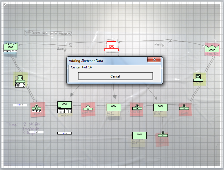
Auto-adding data
So copying data from the image can be pretty tricky, usually because it's hard to read handwriting when the pictures are usually taken from somewhat far away. Also the transparency doesn't help, but turning off the Visio grid can help. But we usually will just go post-it by post-it, and enter data.
After your sketch is complete, you can complete the transformation to a regular map, by using the Sketcher Align tool, which is also currently only in the Beta toolbar. This tool tries to recognize the spatial relationships between all the Sketcher shapes on the page, and lay the map out for you as you would if you had just used our quick stencils.

Aligned map
The Sketcher Align tool used to be in the main toolbar, but during our training sessions users really really hated it, but I think we've improved it since then. Once we got Undo to work with it, I think it became a little more popular, since it's not always great at aligning things. One thing to note here is, I actually copied the Sketch onto a new page, without the post-it picture as a background.
Thursday, November 14, 2013
eVSM Beta Toolbar
One thing we haven't previously made public (that I'm aware of), is a beta toolbar/ribbon in eVSM v6. This is where we keep some tools/features we're working on that aren't quite done yet. Sometimes they are done, and we don't believe them to be mainstream enough to warrant taking up space in the main eVSM ribbon/toolbar.
So with every copy of eVSM v6 we ship two ribbon/toolbar files, in the Program Files\eVSM\Setup\Solutions folder. The main ribbon is stored in the eVSMIconsLGR.xml, and contains the data for building just the main eVSM toolbar.
The second file, when shipped, is called eVSMIconsLGRDev.txt. If you want access to the beta ribbon, just rename that file's extension to XML, and the next time you start eVSM you'll see two new ribbons/toolbars in addition to the main eVSM ribbon. One is the eVSM Beta ribbon, and the other is a Developer Tools ribbon, for anyone who wants to build their own stencils.
I will start writing up some of the tools in the beta ribbon soon. Until then feel free to look around at them and if you want to know more about them feel free to contact me.
So with every copy of eVSM v6 we ship two ribbon/toolbar files, in the Program Files\eVSM\Setup\Solutions folder. The main ribbon is stored in the eVSMIconsLGR.xml, and contains the data for building just the main eVSM toolbar.
The second file, when shipped, is called eVSMIconsLGRDev.txt. If you want access to the beta ribbon, just rename that file's extension to XML, and the next time you start eVSM you'll see two new ribbons/toolbars in addition to the main eVSM ribbon. One is the eVSM Beta ribbon, and the other is a Developer Tools ribbon, for anyone who wants to build their own stencils.
I will start writing up some of the tools in the beta ribbon soon. Until then feel free to look around at them and if you want to know more about them feel free to contact me.
eVSM v6.31 Released
eVSM v6.31 was recently released, which includes some updates to several quick stencils, as well as some bug fixes in the software, and a little change to the XY Chart. The XY Chart now allows you to plot as a horizontal bar chart or vertical, with the default being vertical.
Friday, November 1, 2013
eVSM v6.30 Released
Monday, August 19, 2013
Pizza Tracker
Good article about how Domino's pizza tracker works from within the kitchen. Interesting to think about how well the employees might remember to update the trackers, and how you might approach something similar in a manufacture-to-order environment. What about in health care?
http://www.shmula.com/wheres-my-pizza-behind-the-scenes-at-dominos/11659/
http://www.shmula.com/wheres-my-pizza-behind-the-scenes-at-dominos/11659/
Wednesday, June 12, 2013
eVSM Managed Equations - What They Are and How They Work
This is going to be the first of several posts detailing how to use managed equations in eVSM v6. This will mostly apply to v5 as well, but v6 has added a few extra selectors that I will be going over.
Before eVSM v5, any user wishing to calculate variables in a map had to do so themselves. This entailed building a map, then running the Excel calculator to populate a worksheet with all the variables on the map. Then, the user could build equations using Excel's standard equation editing capabilities. If you had to add more activities to a map, you had to re-run the calculator, then either re-apply an equation you already wrote, or write it fresh to work with the new activities.
Around v5.18 (this was before my time with the company) eVSM added what are called Managed Equations. Managed Equations are kind of meta-level equations, specifying how to build Excel formulas, based on what data is available within a map. More specifically, a Managed Equation tells the eVSM calculator engine how to build an equation for a particular variable on a particular IsARow shape.
An IsARow shape is just a shape that gets its own row in Excel. Any IsARow shape needs to have an operation tag glued on in order to go to Excel (except for arrow data, which I'll get to). So when I say IsARow, I mean an activity block or inventory shape or whatever, which has data blocks glued on.
This Managed Equations capability allows the developers of eVSM to produce standardized templates, with predefined variables, that automatically get calculated. So long as you stick to the standard naming convention, eVSM is able to automatically figure out your equations for you.
So, to get into how Managed Equations work, I'm going to introduce a very simple example, below:

Before eVSM v5, any user wishing to calculate variables in a map had to do so themselves. This entailed building a map, then running the Excel calculator to populate a worksheet with all the variables on the map. Then, the user could build equations using Excel's standard equation editing capabilities. If you had to add more activities to a map, you had to re-run the calculator, then either re-apply an equation you already wrote, or write it fresh to work with the new activities.
Around v5.18 (this was before my time with the company) eVSM added what are called Managed Equations. Managed Equations are kind of meta-level equations, specifying how to build Excel formulas, based on what data is available within a map. More specifically, a Managed Equation tells the eVSM calculator engine how to build an equation for a particular variable on a particular IsARow shape.
An IsARow shape is just a shape that gets its own row in Excel. Any IsARow shape needs to have an operation tag glued on in order to go to Excel (except for arrow data, which I'll get to). So when I say IsARow, I mean an activity block or inventory shape or whatever, which has data blocks glued on.
This Managed Equations capability allows the developers of eVSM to produce standardized templates, with predefined variables, that automatically get calculated. So long as you stick to the standard naming convention, eVSM is able to automatically figure out your equations for you.
So, to get into how Managed Equations work, I'm going to introduce a very simple example, below:
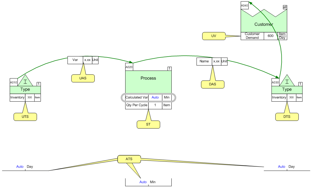
In this example I have a Process box at tag A020, with a variable attached called Calculated Var. There is an inventory block upstream at tag A010, which is connected to tag A020 with a Tag Sequence Arrow. This arrow denotes a flow between A010 and A020. Attached to that arrow is a Short NVU variable, just called Var.
Also, there is an inventory block downstream from the A020 tag, at tag A030. There is a Tag Sequence Arrow denoting flow between A020 and A030, with a Var variable on the arrow as well. Lastly, there is a customer center at tag A040, with a Tag Sequence Arrow connecting tags A030 and A040.
So let's say that we assume that anywhere we have the "Calculated Var" variable, we want to calculate the variable to be the quotient of the Qty Per Cycle for the same activity and the upstream inventory, divided by the product of the Customer Demand and the total Value Added and Non Value Added times for the map.
To start off, we'd have to open the eVSM Name and Unit Manager, which is the XYZ button in the toolbar/ribbon, depending on what version of eVSM you're using. You then just click the Equation Manager, and either edit an existing equation or create a new one. Equations are named after the variable that is being calculated, and there can only be one equation per variable name. Also, the variable must be defined before you can create an equation.

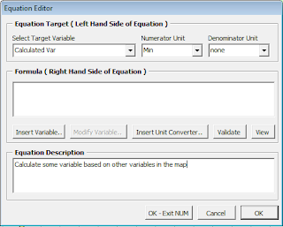
So the Equation Editor above shows that I've selected the Calculated Var as the Target Variable. The Target Variable is just the variable name that is getting calculated. eVSM automatically populates the Numerator and Denominator unit for the Target Variable. This is the unit the equation should calculate to. If your equation calculates to Minutes, but you have Hours selected on the actual variable shape, eVSM will automatically convert the unit for you. My point here is, you should only use unit converters explicitly in a managed equation if the default units for different variables don't match up.
So setting up the new equation is pretty simple; you just select the Target Variable, and populate the Right Hand Side of the equation (RHS). The RHS is the actual calculation to take place.
There can be three different components in the RHS: a Variable Selector, a unit converter, or Other text. These components together will be used to build an Excel formula. The Other text pieces get used to build up more complex Excel formulae, unit converters get used to convert terms to the correct units, and Variable Selectors get used to aggregate a set of variable cells into a single number.
The Variable Selectors are the most complex part of a managed equation, so I'll start there, and the Other text and unit converters should start to make sense, too.
A Variable Selector is a text representation for searching for data somehow related to the target variable. Going back to the example above, you might notice a few different possible relationships between the Calculated Var variable and other variables on the map:
- the "Qty Per Cycle" variable is connected to the same IsARow shape as the target variable, and so we call that relationship ST for Same Tag
- the Inventory variable on tag A010 is connected to the target variable, via the Tag Sequence Arrow. Since the A010 tag is on the upstream side of the arrow, the Inventory variable is then considered a UTS variable, for Upstream Tags. One thing to note is, you may have multiple inventory centers upstream from the activity, each with an Inventory variable, and so the UTS selector would return all of those Inventory variables.
- the Inventory variable on tag A030 is connected to the target variable, again via a Tag Sequence Arrow, but this time the Inventory variable is on the downstream side of the arrow. So this relationship, from the perspective of the Target Variable, is DTS, or Downstream Tags. Again, this selector could return multiple Inventory variables.
- the Customer Demand variable is not directly connected to the A020 activity at all. Instead this is sort of a map-wide value, so it shouldn't be considered to be connected to any IsARow shape or variable (it is connected in this map from the A030 tag, but that's more of a visual representation of flow). So the selector to use to grab a variable from anywhere on the page is UV, for Unique Variable.
- The Non Value Added variables on the two inventory tags are technically connected through a UTS and DTS relationship, technically. But, if you wanted to get all the Non Value Added variables for the entire map, you would use the ATS, or All Tags, selector to get those. ATS will just return the set of all Non Value Added variables on the whole map, regardless of tag sequence.
So these are the five most basic selectors available in eVSM. This is already getting really long, so I'll move on and cover the remaining selectors in a future post. These other selectors mainly relate to getting data from the middle of a tag sequence or pipe arrow, or having the target variable reside in the center of a tag sequence or pipe arrow.
Next I want to mention the impact of eVSM Paths on managed equations. The eVSM calculator engine first evaluates the selectors (for instance, you want Non Value Added from All Tags (ATS)). So the calculator engine gets the set of all Non Value Added variables on the map, and for each one looks at whether there is a path match between the target variable's IsARow shape, and the candidate selector variable's IsARow shape. If one of the IsARow shapes is on the All path, then it's just accepted, but if not then we check each path between the IsARow shapes. If no match is found then it is removed from the selector set.
So at this point in the calculation, the selector has returned a set of variables, which need to be aggregated in some way. To aggregate the set to a single number, we can apply one of a number of Excel functions: SUM, AVERAGE, COUNT, MIN, MAX, or PRODUCT. So once the selector returns the set of variables for the term, the calculator engine converts that set to text, as, for example, "SUM(A010 Inventory,A020 Inventory)". Instead of putting in "A010 Inventory", we actually put the Excel address of A010's Inventory variable (so "E5" if A010 is in row 5, and Inventory goes into column E).
So that's for a scenario where the selector returns one or more variables. If a selector returns no variables, then the calculator goes into the Apply/Skip phase. Basically, for each term you have to specify what to do if the selector returns an empty set. You can Skip the equation, which means the calculation engine will not apply any Excel equation, instead just using the current text in the target variable shape. Or, you can elect to apply a default value, which is usually just zero, but can be any number.
So that explains how each term/selector gets evaluated on its own, so I'll now go into how this all works into a managed equation. Rather than start with my ridiculous example, I'll first pull a real-world example from eVSM's Quick Manufacturing template.
The example I'll use is the Activity NVA Per Unit equation, below:
ST(Activity NVA;Min;0;SKIP)/(ST(Qty Per Cycle;Item;1;APPLY)*ST(Stations;Stn;1;APPLY))
I've highlighted the three different selectors in this equation in yellow, and the light blue text is considered Other text.
The equation spreads the Activity NVA value on an IsARow out over the different stations performing the activity, and across multiple parts per activity run.
So let's break down the different selectors, which are all pretty basic:
- ST(Activity NVA;Min;0;SKIP) - This selector is looking for the Activity NVA variable on the same tag as the target variable. It is expecting the value to be in Minutes, and if no Activity NVA variable is found on the same tag, then we skip the equation.
- ST(Qty Per Cycle;Item;1;APPLY) - This selector is looking for a Qty Per Cycle variable on the same tag as the target variable, in units of Item. If the variable is not found, then we just assume a value of 1.
- ST(Stations;Stn;1;APPLY) - This selector is looking for a Stations variable on the same tag as the target variable, in units of Stn. If it's not found, we assume a value of 1.
So when this is being applied to an IsARow with Activity NVA of 5 Min, Qty Per Cycle of 3 Item, and 3 Stations, the resulting equation would have the selectors just replace with cell addresses, and we'd be left with something like: D5/(E5*F5). As you can see by the blue highlighted text in that resulting formula, we literally just put in whatever text we classified as "Other". In this case, it's simply specifying an order of operations with different operators and parentheses.
However, in Quick Manufacturing, we do get a little more complicated with some of the "Other" text, though the logic here is pretty straightforward. As an example, I'll use the Computed Activity Time equation:
if(ST(Activity Time;Hr/Day;0;APPLY)=0,CONV(DAY;Hr),ST(Activity Time;Hr/Day;0;APPLY))
I've used the same color scheme, though I did add the magenta color for the unit converter. But you can see here we're using Excel's IF function, but the meaning may not be immediately straightforward. A different way to read this equation may be:
If the Activity Time on the same tag as the target is zero, use the conversion factor between days and hours, otherwise use the Activity Time variable value. So the conditional portion of the IF function is simply allowing us to use a selector to govern the logic of the calculation. This is just a simple example, but you may see this in use in other built-in equations. The thing to keep in mind is, this is how the developers of the stencils make the calculations smart enough to recognize whether certain variables exist on an IsARow, and kind of a chain of ways to handle the different scenarios.
So now my crazy example from above should be relatively easy to piece together, with knowledge of the different selectors in eVSM. First, I'll write out the equation in relatively plain English:
the quotient of the Qty Per Cycle for the same activity and the upstream inventory, divided by the product of the Customer Demand and the total Value Added and Non Value Added times for the map.
So that to me means we want to have something like:
(ST(Qty Per Cycle)/UTS(Inventory))/(UV(Customer Demand)*((ATS(Value Added)+ATS(Non Value Added)))
In the above, I've simply tried to match text formatting to show the different parts of the equation. This is almost complete; we just need to specify units, aggregation functions, and Skip/Apply options:
(ST(Qty Per Cycle;Item;0;APPLY)/UTS(Inventory;Item;0;APPLY;SUM))/(UV(Customer Demand;Item/Day;0;SKIP)*((ATS(Value Added;Min;0;APPLY;SUM)+(ATS(Non Value Added;Min;0;APPLY;SUM)))
So at first glance, these equations may look very complicated, but the key to understanding them is to break them down into the individual pieces: Selectors, Converters, and Other text. The Other text will give you a clue as to the intention and logic of the equation, and the selectors are just finding data in relation to the variable shape being calculated.
I'll go into the remaining selectors, as well as our calculation debugging efforts, in a future post.
Thursday, April 4, 2013
More on the new eVSM Calculator Engine
In my last post I talked about the new eVSM Calculator engine. I mentioned how this new more flexible engine allowed us to do some cool new things, and I'd like to go over some of those cool things here.
The first new tool is the Source/Target capability in v6 (I think available after 6.15 or so). Source/Target is simple enough in principle, in that it simply enables you to link a variable shape to one or more other variable shapes. This actually works between pages in a single Visio document, so you can cross-link from one map to another.
Here are the shapes you use:
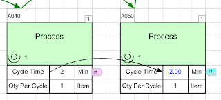 The pink shape is a Data Source, and is basically a named variable on the map. You just specify a short alphanumeric name for the source, and then you add one of those blue shapes, called a Data Target. You just make the link by making the target name the same as the source name.
You can actually have multiple data sources with the same name, and if you look closely at the target shape it says "SUM". This is the default way the target handles multiple data sources: it sums their values. If you right click the target shape you can change it to take the average, max, or min value of the sources available with that name.
You can also make the target path-based, meaning it only uses sources that are on centers with the same path number. There's also a new (in v6.20) option when you right click a target shape for viewing the sources that the target will use.
One important note here is that by default, the calculator engine will only search the current map, for data sources and targets. If you want to link to another page, you have to set the "Page Scope", so that the calculator engine knows what pages to search. We do this because we actually calculate each page in the scope, in order to make sure the values we use are current. We also do this because if you copy a map to build a future state map, your source and target names would stay the same, and so we'd actually start using a lot of data we shouldn't.
To modify the Page Scope, click the Name Unit Manager button in the eVSM Toolbar/Ribbon, and click "Page Link Scope" near the bottom. You'll then see a list of all the pages in the current document, except for the current page. We don't list the current page since it's included in the page scope by default.
Now, here are some advanced tips for using source/target:
The first new tool is the Source/Target capability in v6 (I think available after 6.15 or so). Source/Target is simple enough in principle, in that it simply enables you to link a variable shape to one or more other variable shapes. This actually works between pages in a single Visio document, so you can cross-link from one map to another.
Here are the shapes you use:

You can actually have multiple data sources with the same name, and if you look closely at the target shape it says "SUM". This is the default way the target handles multiple data sources: it sums their values. If you right click the target shape you can change it to take the average, max, or min value of the sources available with that name.
You can also make the target path-based, meaning it only uses sources that are on centers with the same path number. There's also a new (in v6.20) option when you right click a target shape for viewing the sources that the target will use.
One important note here is that by default, the calculator engine will only search the current map, for data sources and targets. If you want to link to another page, you have to set the "Page Scope", so that the calculator engine knows what pages to search. We do this because we actually calculate each page in the scope, in order to make sure the values we use are current. We also do this because if you copy a map to build a future state map, your source and target names would stay the same, and so we'd actually start using a lot of data we shouldn't.
To modify the Page Scope, click the Name Unit Manager button in the eVSM Toolbar/Ribbon, and click "Page Link Scope" near the bottom. You'll then see a list of all the pages in the current document, except for the current page. We don't list the current page since it's included in the page scope by default.
Now, here are some advanced tips for using source/target:
- Every variable shape on the map actually has a "hidden" Data Source shape on it, with the variable name as the text. So if you wanted to simply put the sum of all Cycle Time variables in the Lead Time variable, you would just add a Data Target to the lead time and set its text to Cycle Time, and that's it!
- The source/target engine uses text matching to find matches, so not only are they case-insensitive, you can use simple wildcards to make the target a bit more flexible. For instance, if you had three sources, S1, S2, and S3, you could get the Sum of all three by setting your Data Target text to "S*". The * character tells us to just look for the letter S followed by anything. You could also do "S#", which would only match the letter S followed by a single number.
Source/Target gives eVSM users a powerful method for linking between maps, especially with our new Wizards we are creating (I'll talk about those in the future). If you're curious, you can actually see that the way this works is very simple. We are just linking cells in the eVSM document's Excel workbook, the same that you could do manually. This is just a way for you to tell eVSM to make those links.
Subscribe to:
Posts (Atom)